
Froude theory for propulsion and traction propellers
Froude theory for propulsion propellers shows that creating thrust means accelerating a flow of fluid. It puts a number on it: thrust equals the mass flow rate crossing the propeller times the acceleration it gives the fluid, T = ṁ (V2 − V0), and the velocity at the disc is the mean of the upstream and downstream velocities. This page establishes these results with all their formulas. It relies on the momentum balance.
In this page:
- Froude theory: the propeller seen as a disc
- Momentum balance
- Pressure and induced velocity at the disc
- Propeller thrust formula: mass flow and acceleration
- Worked example: thrust and Froude efficiency
- Limits of the theory
1: Froude theory, the propeller seen as a disc
Froude's approach evaluates the axial induced velocity with a control volume around the stream tube crossing the propeller. The propeller accelerates the fluid, the tube contracts, and fluid must therefore enter the control volume sideways to compensate. We can compute that volume.
Following Froude, we regard the propeller as a uniformly loaded disc with an infinite number of blades (figure 1). Four assumptions simplify the problem:
- we ignore the rotation of the flow;
- outside the stream tube, the flow is undisturbed;
- the pressure far upstream and far downstream equals the static pressure of the undisturbed flow;
- the disturbances are small enough for the fluid density to be constant.

Figure 1: the accelerated stream tube contracts. On the left, V0 and p0 upstream; at the disc, the pressure jumps from p to p + Δp; on the right, V2 and the tube radius r downstream, inside a volume of radius R.
2: Momentum balance of a propulsive propeller
We write V0 for the velocity far upstream, V1 for the velocity at the disc, V2 for the velocity far downstream, r for the radius of the stream tube far downstream and R for the radius of the control volume. The continuity equation gives the volume flow rate Q crossing the outer surface of the control volume:
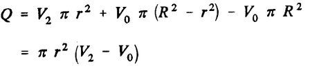
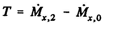
The momentum theorem gives the traction (or propulsion) force T of the propeller, that is the change of momentum between sections 2 and 0, projected on the horizontal axis:
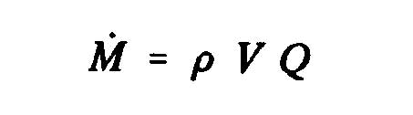
The time derivative of the momentum is:
The momentum M2 leaving the control volume at section 2 is:

The total momentum M1 entering the control volume is the momentum at the volume inlet, plus the momentum entering sideways:

The axial force (T = M2 − M1) therefore becomes, with the simplification on the second line:

3: Pressure and induced velocity at the propeller disc
The traction force can also be written with the resultant of the static pressure on the disc:
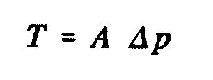
where A is the area of the disc swept by the propeller and Δp the pressure difference across the disc. The Bernoulli equation reads, from 0 to 1 upstream:
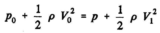
and from 2 to 1 downstream:
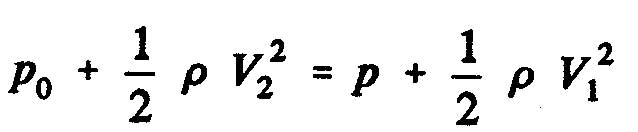
The static pressure difference between the downstream and upstream faces of the disc is:

The continuity equation between the disc and section 2 reads 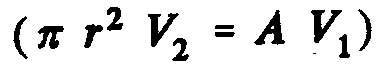 , which allows us to write:

We conclude that the flow velocity at the disc is the arithmetic mean of the upstream and downstream velocities:
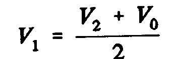
The induced velocity, written w, is the increase of velocity at the disc, and a is the axial interference factor:
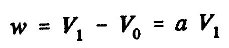

Reading note: these two images mix two conventions for a. Since V1 is the mean of V0 and V2, the induced velocity is w = V1 − V0 = V2 − V1 = (V2 − V0)/2. With the usual definition a = w/V0, we have V1 = (1 + a) V0 and V2 = (1 + 2a) V0. This is the convention of the page on induced velocity, where the axial velocity seen by the blade is V(1 + a).
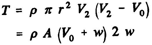
With the mean , the traction force acting on the disc is:
4: Propeller thrust formula, mass flow and acceleration
This expression of the thrust brings out the mass flow rate. The mass of fluid crossing the propeller per second is, in kg/s:
ṁ = ρ A V1 = ρ π r2 V2
with ρ the density in kg/m3, A the disc area in m2 and r the radius of the stream tube far downstream (section 2), in metres. The thrust of the propeller is then:
T = ṁ (V2 − V0)
Creating thrust therefore means increasing the velocity of a mass flow of fluid. We have two levers, the mass moved or the acceleration given, and the choice between them is decisive for the propulsive efficiency.
5: Worked example of thrust, induced velocity and Froude efficiency
The values below are an example chosen to illustrate the formulas; they are not measurements. Take a propeller 2 m in diameter advancing at V0 = 20 m/s in air (ρ = 1.225 kg/m3), and assume the propeller imposes an induced velocity w = 3 m/s at the disc.
- The disc area is A = π × 12 ≈ 3.14 m2.
- The velocity at the disc is V1 = V0 + w = 23 m/s, and the velocity far downstream V2 = V0 + 2w = 26 m/s.
- The mass flow rate is ṁ = ρ A V1 ≈ 88.5 kg/s.
- The thrust is T = ṁ (V2 − V0) = 88.5 × 6 ≈ 531 N. The formula ρ A (V0 + w) 2w gives the same result.
The useful power, the one that moves the vehicle, is T × V0 ≈ 531 × 20 ≈ 10,620 W. The power given to the fluid is T × V1 ≈ 531 × 23 ≈ 12,215 W, which ½ ṁ (V22 − V02) confirms. The difference, about 1,590 W, is the kinetic energy left in the wake. The ratio of the two is the Froude efficiency (ideal efficiency): η = V0 / V1 = 20 / 23 ≈ 0.87.
This efficiency shows the lever mentioned above. For the same 531 N of thrust, a propeller twice as large would move almost twice the flow and need almost half the acceleration: V1 would come closer to V0 and the Froude efficiency would rise. This is why slow, large-diameter propellers are more efficient than small, fast ones at equal thrust. At zero forward speed (static thrust), η falls to zero: the thrust is real, but the useful power is zero, because nothing moves forward.
6: Limits of Froude theory for a propulsive propeller
This efficiency is a ceiling, not a forecast. The theory contains neither airfoil drag nor wake rotation: a real propeller spins the fluid, and the energy of that rotation is lost on top of the axial acceleration. It also assumes an infinite number of blades, hence no tip loss, and a uniform flow over the disc. A real propeller therefore stays below the Froude efficiency, all the more so as the rotation is strong, that is at low forward speed and high torque.
To know which blade shape actually produces this thrust, we need blade element theory for a propulsive propeller, which brings in the airfoils and their Cl and Cd. For its wind turbine counterpart, see BEM for energy-capturing rotors.
Froude theory gives the axial induced velocity. Coupled to blade element theory, it splits this induced velocity into axial and tangential components, which are needed to predict angles of attack and blade geometry.
To go further, we can look at the blade element calculation for propulsion propellers, the energy-capturing case with the Betz limit, or the bibliographic references.
 Global site map
 Mecaflux
 Tutorials Mecaflux Pro3D
 Tutorials Heliciel
 Tutorials Heliciel PRO CFD
 Mecaflux Store
 Compare software functions
 Quotes, Orders, Payment Methods
 project technical studies